This tutorial explains how to interpolate a "synthetic" color channel from two existing color channels. (If you're unfamiliar with how spacecraft make color images, read this) Incomplete color coverage is relatively common and in most cases, an intentional outcome. Data budgets are relatively tight for a number of reasons: onboard space is limited, transmission is slow, and ground stations for reception are heavily booked. If a color filter doesn't add useful information for a researcher, sending back data taken with that filter doesn't make a lot of sense.
Interpolation makes use of a relatively safe assumption in color processing. Most planetary surface surfaces show relatively gradual changes in the way they reflect light. If an object is bright at red wavelengths and dark at blue wavelengths, then we can assume that its brightness will be somewhere in between at green wavelengths. So, if "green" is located halfway between the spectral ranges of a red filter and a blue filter, then simply averaging the two pictures should accurately recreate what the surface would look like if we had actually taken a picture with a green filter. This assumption is frequently used by spacecraft imaging scientists, because it means they can remove the green filter entirely and replace it with another filter that will provide more information. (This is why the New Horizons MVIC camera did not have a green filter!) We can extend this assumption to deal with any filter combination within a spacecraft's filter range. However, as we get out into the near-infrared or near-ultraviolet, planetary surfaces start to show strong variability over short wavelength ranges. That means our assumption may be inaccurate, and we're not actually replicating what a surface might look like.
This tutorial uses Photoshop CC, but uses features that are standard in most photo editing software.
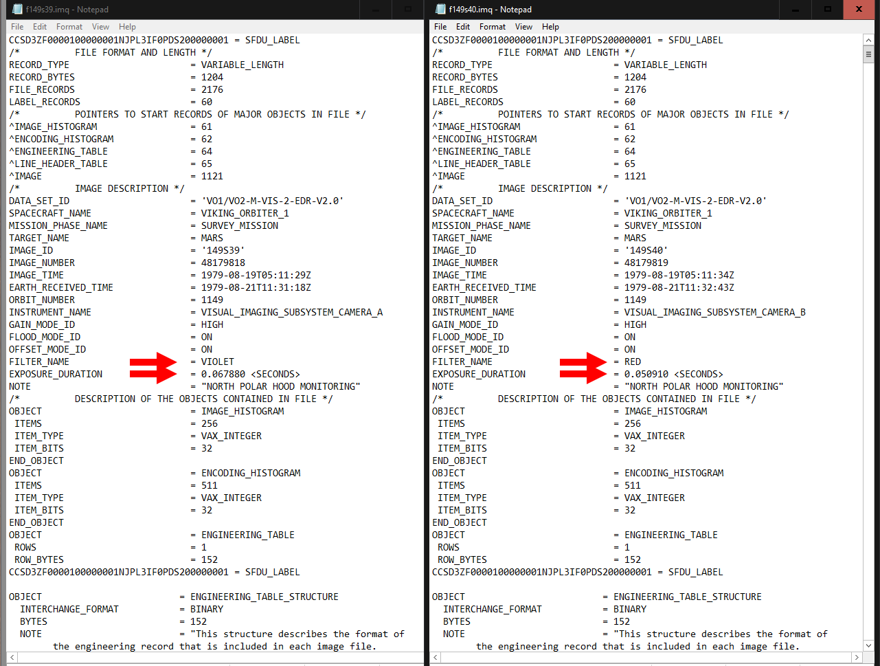
For this tutorial, we wil be using a red-violet pair of images taken by the Viking 1 orbiter (f149s39 (violet filter) and f149s40 (red filter)). The links to be taken to a page with the full-resolution images.
Our first step is to calculate the photographic stop between of the different images. Looking at the associated label file for the images, we can see that the exposure length was 0.067780 s for the violet filter image and 0.050910 seconds for the red filter image.
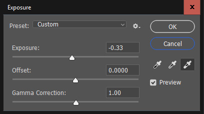
We'll calculate stop in terms of the red image. Divide 0.67780 by 0.050910, and we get 1.33. This is 1/3 of the way between 1 and 2, so that corresponds to a stop of +0.33. On the violet image, go to Image -> Adjustments -> Exposure. In the exposure field, adjust the value to -0.33. Now the brightness of the violet image is the equivalent to an exposure of the same length as the red image.
The next step is to align the images. For this image set, Photoshop's "Auto-Align" feature can get the features pretty close (to do this, select both images as layers, then go to Edit -> Auto-Align Images). However, we still need to make some small adjustments with the transform tools (Edit -> Transform -> Distort [or Warp]). Getting a perfect alignment is absolutely critical, or else we will end up with green and magenta color fringes around sharp boundaries later on. When I am processing color images, I spend more time on this step than anything else.
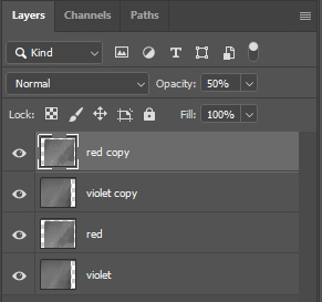
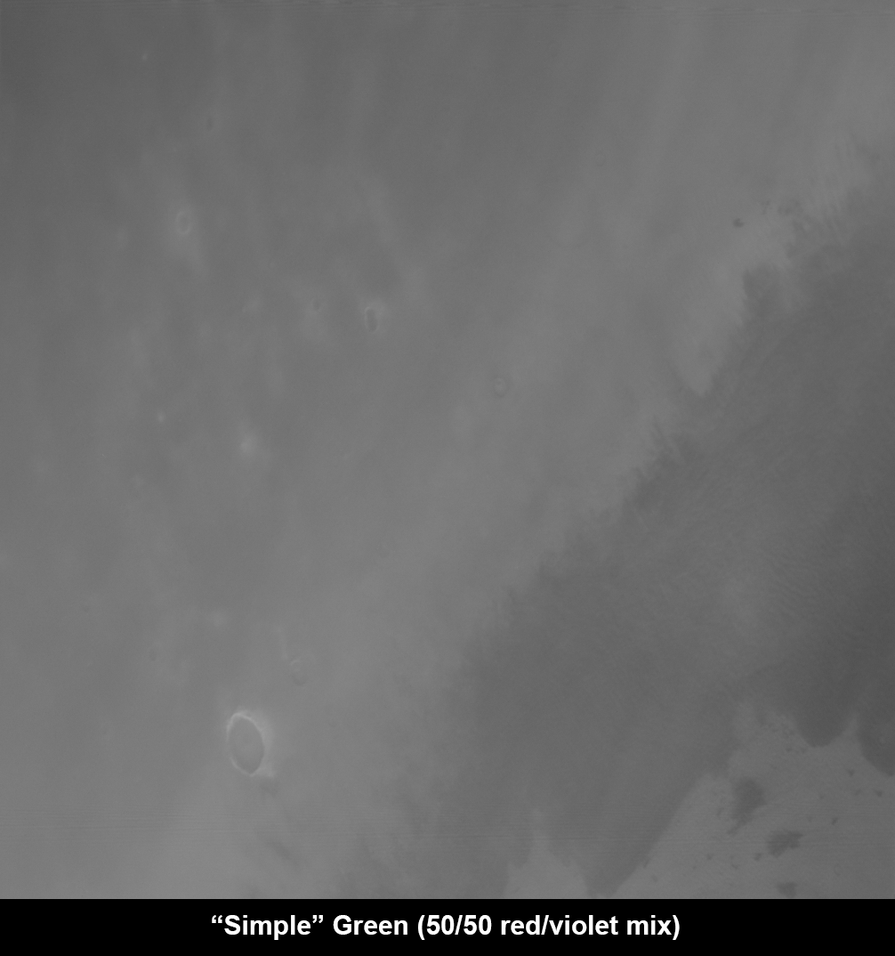
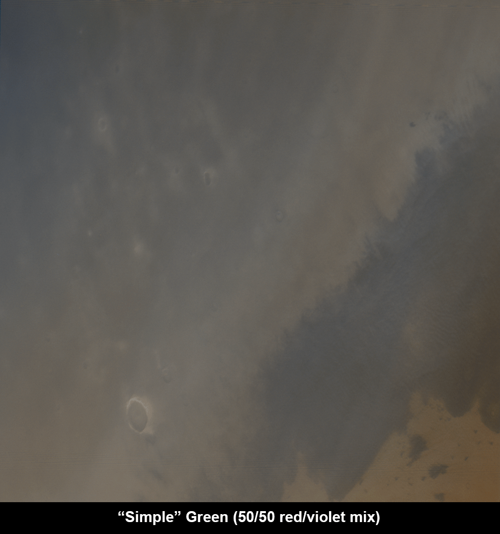
Now we're ready to make a synthetic green filter. We can do this a couple of different ways. The simple way is to simply average the two frames. This approach has simplicity on its side, because it doesn't require much messing around with filter responses and band math. Duplicate the two color layers, and set the red image to 50% opacity.
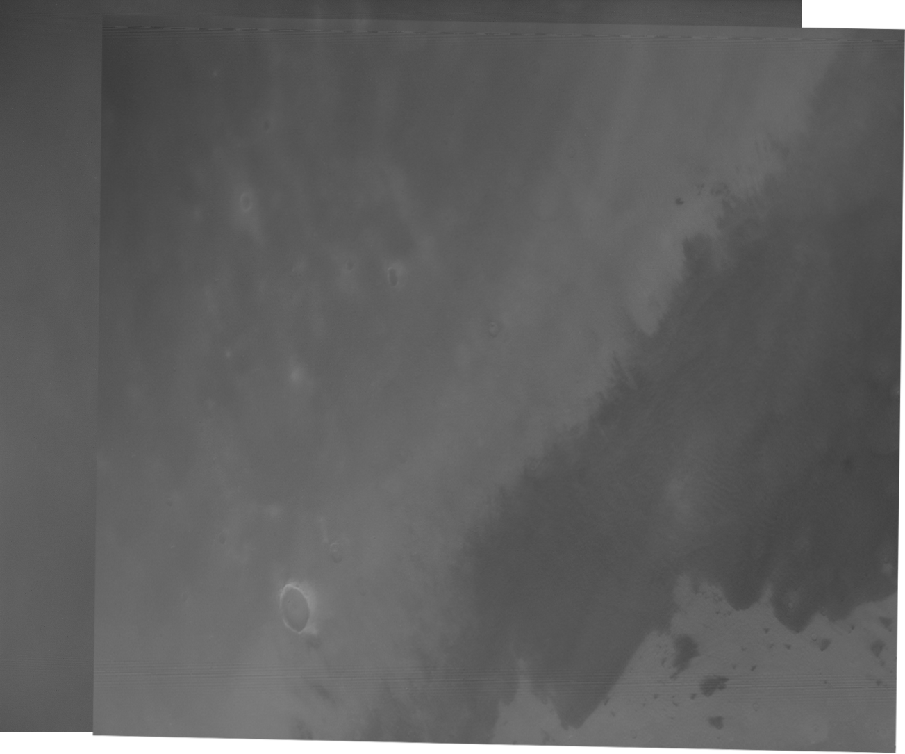
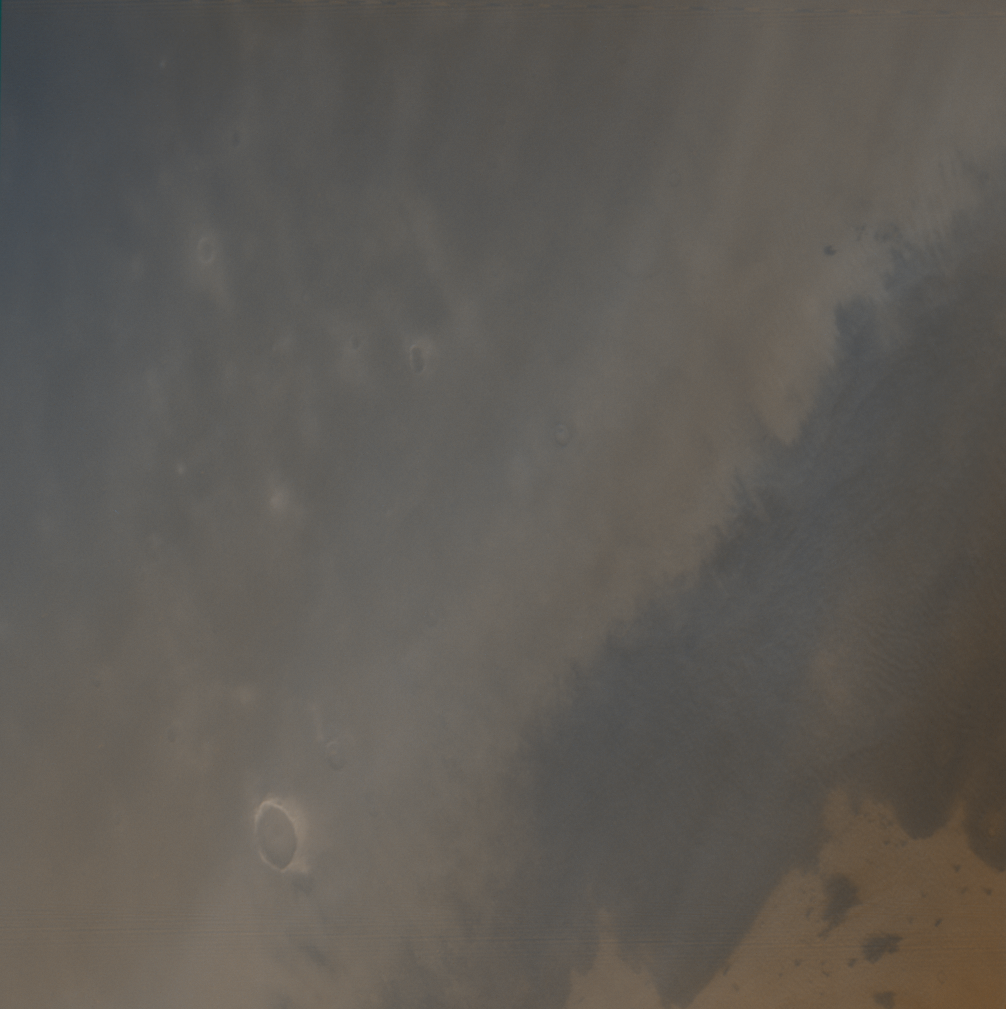
Here's what a color image using the synthetic green filter will look like after cropping out the parts where images don't overlap with one another:
This is a perfectly fine place to stop. If you want to continue on into the weeds of more accurate color, read on...
We can actually make our interpolated slightly more accurate to the Viking filter responses. Let's look at the wavelength ranges covered by the spacecraft fitlers. The violet filter is centered at 410 nm, and the red filter is centered at 625 nm. Our simple 50-50 average above effectively results in a synthetic green filter centered at 517 nm - a little bluer than Viking's green filter (550 nm). To accurately replicate the green filter, we need a weighted average that slightly prefers the red filter. Solving for the weighting factors that give us an average of 550 nm, we find that it is ~0.35 violet, ~0.65 red. So, we'll set the opacity of the red layer to 65% instead of 50%.
Comparing the "simple" synthetic green and the "Viking" synthetic green, the changes are very subtle, with slight changes in color of very light and very dark surfaces. This isn't surprising, because Mars' surface shows more contrast at red wavelengths. Because our "Viking" green uses more of the red filter than the "simple" green, we see slightly higher contrast in the "Viking" green.
Applying that result to the three-color image, we see that the image overall looks a little greener. That's because the "Viking" green is weighted a little more towards the brighter red image than the "simple" green. Because the green channel also has slightly more contrast, we can see that bright areas a little greener (we added more green), and dark areas are a little more pinkish (we subtracted greeen, giving us magenta).
For most purposes, I prefer to just go ahead and use the "simple" green, because for most data sets the difference isn't all that large. Although it might be slightly more accurate, I don't feel like spending the time calculating weights.