This tutorial applies the technique of image differencing to searching for dust devils in Mars rover data. Although Martian dust devils can look as spectacular as their terrestrial counterparts, in most regions the thin atmosphere has a difficult time lifting enough dust to make them visible. At Curiosity's home in Gale Crater, dust devils typically only reflect ~1% of the light hitting them. This makes them nearly transparent, requiring enhancement to be made visible.
As part of its goal to provide information on the Martian atmosphere, Curiosity regularly perform dust devil watches. These watches repeatedly image a region (typically 10-20 times) over the span of a few minutes. This process relies on chance, and so many of these watches come up empty-handed. But every now and again, the rover gets lucky and catches a passing dust devil. This processing tutorial uses a successful dust devil watch performed on Sol 2310, which successfuly captured a large dust devil moving through the hills on the lower slopes of Mt. Sharp.
The tutorial is adopted from techiques used by professional researchers to study Martian dust devils. It uses Photoshop CC, but uses standard features in most photo editing software.
Our first step is to create a reference image. In dust devil watches, we don't know ahead of time which frames contain a dust devil and which ones don't. If our reference image contains a dust devil, it will show up in every frame we try to difference! To get around this, we'll combine all of the images taken during the observation. Here, we'll do this by applying a median filter. I prefer using the median because a given pixel will vary by only 1-3 DN values due to noise throughout an observation. A dust devil will be far from the median value, so this filter will completely remove its presence from the reference frame. An average will greatly reduce the visibility of a dust devil, often below the image's noise floor, but it is good practice to remove as much of the target signal as possible from the reference image.
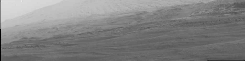
Raw frame from the observation
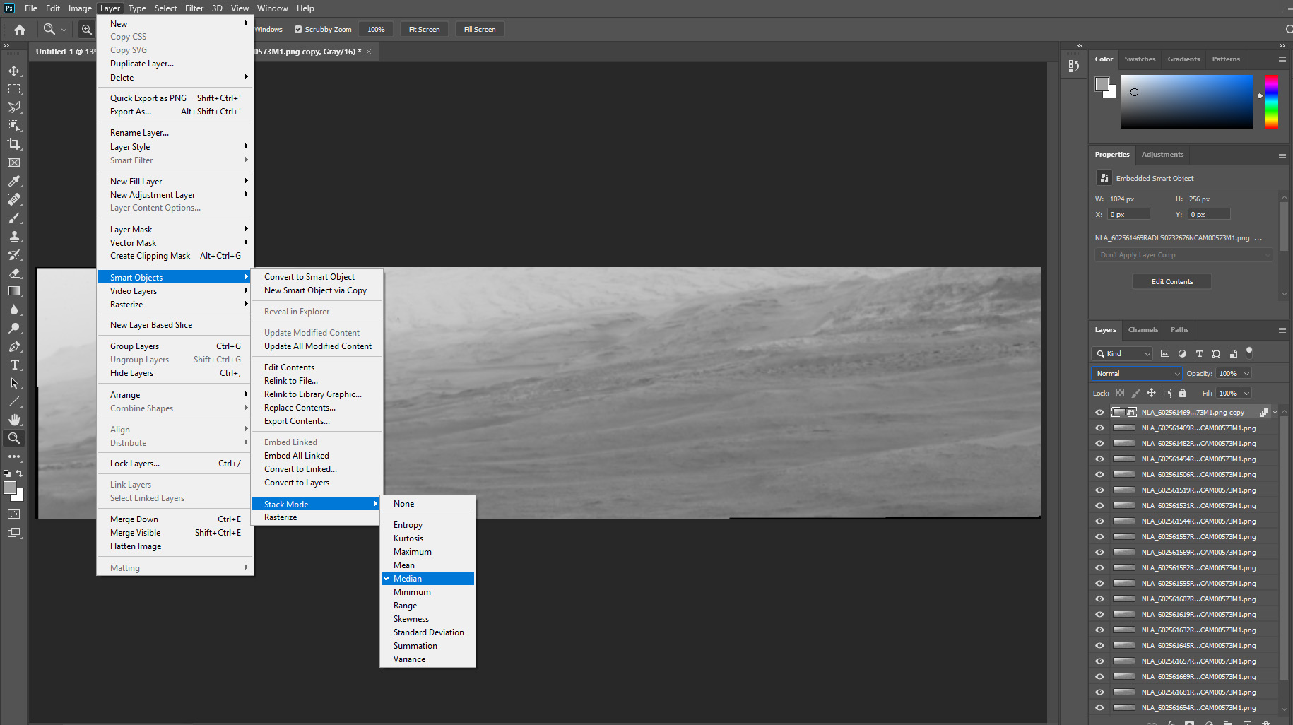
In Photoshop, load all of the images into layers. We'll need to use these images again later, so let's go ahead and select all of the layers, right-click, and select "Duplicate Layers". Then select the new layers, right-click again and select "Convert to Smart Object". On the toolbar, go to Layer -> Smart Objects -> Stack Mode -> Median. This will find the median DN value for each pixel and construct a new image with those DN values. This will be our reference image.
Our next step is to perform the differencing operation using our reference image. Set the blending mode of the reference image to "Difference".
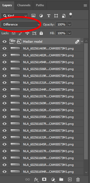
We will need to apply this to every frame in the observation, so let's duplicate all of the raw image layers again, and create a copy of the reference image for each raw image. Then merge each reference-raw image pair with one another, making sure the blending mode for the reference image is set to "Difference". If we flip through the images in the observation, the dust devil pops out very clearly. The first frame catches the initial gust of wind lifting some dust, followed by the development and dissipation of a dust devil over the next few frames.

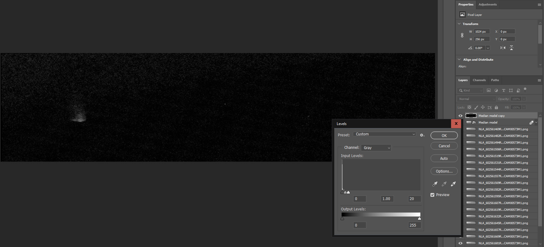
As you can see, the dust devil is very faint, so now we need to do some processing work to make it visible. Go to the toolbar and click Image -> Adjustments -> Levels. This will bring up a histogram of the DN values within the image. We can see a that most of the pixels are around 1-2 DN values. Most of these pixels are just noise! Any signal with this brightness range will be almost impossible to pick out from the noise. So we're simply going to get rid of everything at this brightness level. Drag the slider on the left side of the histogram to 1 or 2. This will set pixels with DN values of 1 or 2 to zero, and darken the remaining pixels by 1 to 2 DN values. There will be some residual speckle noise from hot pixels and a few pixels with unusually high noise, but this should remove most of it.
Now we need to brighten the remaining signal. To do this, drag the slider on the right side of the histogram to ~20. This will scale the pixels with values between 0 (black) and 20 (dark, dark gray) to a new set of values between 0 (black) and 255 (white). Now these differences stand out more clearly. Stretching has the side effect of increasing the visibility of image noise that wasn't clipped by our histogram adjustment, so take care in deciding how far left you drag the slider.
You need to use the exact same stretch on every image in the set if you intend to make a movie! If not, you will end up with flickering brightnesses.
An option for more advanced image processors: the point between discarding noise and rescaling the pixel values is the best time to apply a noise reduction filter to remove remaining speckle. High-contrast speckle noise can be difficult to remove without destroying fine details. Most noise-reduction algorithms seem to handle the speckle a little better when it is low-contrast. My favored choices for noise-reduction at this stage are either the Smooth [Anisotropic] or Smooth [Diffusion] filters in G'MIC for GIMP. But be very careful here. Because the signal is so faint, it is very easy to destroy.
Next, pair off each raw frame with the differenced version of the frame. Set the blending mode of the differenced frame to "Linear Dodge (Add)". This effectively adds the DN values of the two images together. Since most of the differenced image is black, the only change you should see in this blending mode is the addition of the dust devil.
Now for a movie with the processed data: