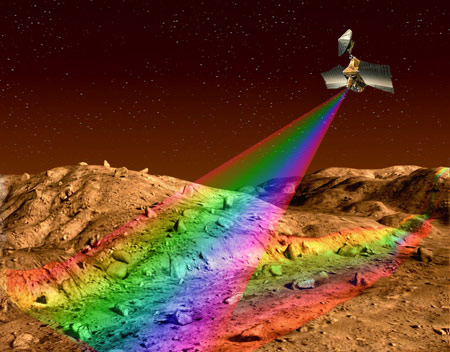
Since 2005, the Compact Reconnaissance Imaging Spectrometer for Mars (CRISM) instrument on the Mars Reconnaissance Orbiter has been collecting data of the Martian surface. CRISM is designed to map out the distribution of different minerals on the Martian surface, and it does this by looking for subtle variations in color. Color is essentially a measure of the relative number of photons reflected or emitted from a material across a given energy range (or spectrum). Individual minerals have a characteristic color based on how their crystal structure absorbs or reflects photons. To human eyes, these differences can be extremely subtle, even invisible - thus the classic warning geology students receive in their mineralogy lab courses: "color is not diagnostic". But strictly speaking, this warning only applies to the human eye - we're only capable of comparing light intensities at three (or fewer) points within a limited region of the spectrum. If we could extend our vision into the infrared, as with an instrument like CRISM, color can be diagnostic.
CRISM is used to highlight minerals of interest, like clays, which may provide clues to Mars' history. I wanted to use CRISM data for a different purpose: approximating human perceptual color from spacecraft data for use in mapping projects. This project began to take shape in August/September 2020, when I decided I wanted to assemble a 5 m/px scale image of Jezero Crater ahead of the Perseverance rover landing. The mosaic would be assembled from Mars Reconnaissance Orbiter CTX images and colorized using lower-resolution data sources like CRISM and Mars Express HRSC. This was actually a second attempt at the mosaic, since I was unhappy with the results of the first attempt.
The first attempt in 2018 had been plagued by several issues that hurt the color quality. The primary issue was getting a visible color image from CRISM in the first place. To explain the problem, I need to back up and explain how the CRISM visible color image was produced in the first place.
CRISM is an imaging spectrometer, which works somewhat differently from a normal camera. At the heart of an imaging spectrometer is a camera sensor. Instead of obtaining color data by rotating a series of color filters in front of the sensor, an imaging spectrometer uses a diffraction grating. The diffraction grating behaves like a prism, splitting the incoming light across the camera sensor. Each row of pixels on the sensor receives light of a different wavelength. The sensor is then scanned across the imaging scene while taking hundreds of images. NASA's "Pluto Through Stained Glass" video nicely illustrates the scanning process at work. Post-processing then slices up the individual images and rearranges them to construct hundreds of single-wavelength images of the target. Each of these sub-images is called a "band", and CRISM has 544 bands in total.
This process creates an image where each pixel contains a spectrum with hundreds of individual points. Math operations can performed on the hundreds of bands can be used to isolate spectral features, like water absorptions associated with clay minerals. This process, called parameterization, reduces the hundreds of points of spectral data down to just a handful of points that are more easily understood. Parameterization is used to produce mineral maps or color composites that provide a representation of the spectral variations present within a scene. One CRISM parameterization is the "visible color" parameter product. This representation is produced by parameterizing regions of the red, green, and blue regions of the visible spectrum. I'll refer to the parameterized images as "channels", as they're analogous to color channels used to construct a color image.
During my first attempt at producing the Jezero mosaic, producing the CRISM visible color parameter product relied on an official instrument toolkit designed to work with ENVI, an expensive geospatial data software suite. Although this was available to me through my graduate work, I did not want to use it as a centerpiece of image processing work, particularly in terms of making processing techniques available for other people to use. Exporting image formats that I could use with Photoshop or another image processing program was difficult with ENVI - it only allowed 8-bit images to be output, and the color range of the output images was limited. As a result, the images tended to be noisy, particularly when larger adjustments were needed to match the brightness and contrast to match another image.
Another issue I had encountered working with ENVI is that the software did not preserve brightness relationships between the individual color channels. This required manually setting the color balance of images by choosing a location in the image where the channel intensities were approximately equal to one another. Not only was this nearly impossible on a reddish surface like Mars, but the method usually washed out the brightest areas of the image. This meant that colors did not output consistently between images, requiring further manual adjustment in Photoshop using another image as a reference.
One last problem that I encountered was inherent to the CRISM image itself. Image spectrometers use a scanning motion to build up the image, and the scanning motion on CRISM incorporated the spacecraft's orbital motion. Towards the start and end of image collection, CRISM was looking at shallower angles through the atmosphere. This meant that more of the signal came from clouds and lofted dust. At the time, the processed images produced by the CRISM team removed only a portion of this signal, often causing the top and bottom edges of the image to be bluer from clouds, and lower contrast due to dust. Beginning in 2016, the CRISM team began applying a more sophisticated image processing routine to remove more of this signal, but these images weren't available in large numbers when I made my first attempt at producing a large mosaic.
The main area of improvement on the CRISM visible color parameter product I had in mind was creating a parameterization that better matched the human color response. Part of the motivation was improving the accuracy of color representations. However, I realized taking this approach would have some knock-on effects which would further reduce color noise present in the CRISM visible color parameter.
A human sees color by processing light received by specialized cells in their eyes. These cells, called cone cells, contain a light-sensitive protein with a structure that is temporarily changed when a photon of the proper energy interacts with it. This stimulates a nerve response which is passed along to the brain's visual cortex. There are three types of cone cells present in the human eye, which are sensitive to different wavelengths of light. The color we perceive is derived by the relative amount of cone cells of each type that are stimulated.
Computing perceptual color requires an understanding of how those proteins are used to perceive color. Colorimetrists have carefully measured the odds that a photon of a given energy will interact with the proteins inside of a given cone cell type, and formed a mathematical description (or "response function"), to describe those odds. The integrated intensity received by each cone cell type is then fed into a mathematical model of how the brain interprets those intensities to produce color. If you're curious to get into more detail of how this is done, I'd recommend reading this very neat article by Douglass Kerr.) The chart below what these response functions look like for the average human eye.
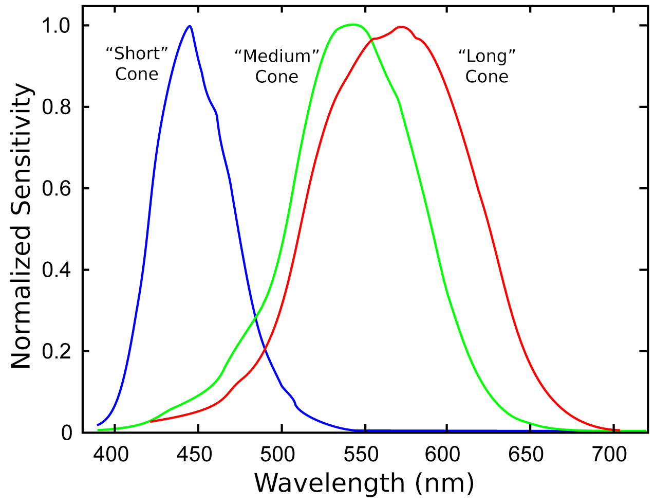
The CRISM visible color parameter image uses a relatively decent approximation for human color vision. It selects regions of the visible spectrum near the effective peak reponses for the "short" and "long" cone cells for the red and blue channels, and near the peak overall sensitivity of human vision for the green channel. The visible color parameter uses the median of five bands to create each color channel, which with the spectral resolution of CRISM corresponds to ~32 nm. Looking at the human visual response functions, we can see that the cone cells are actually sensitive to a larger amount of light, with high sensitivity to at least a 50 nm wavelength range.
This observation meant that by using a human visual response function, we'd be using data from a larger number of bands and effectively reducing the influence of noise present in any one band. My general strategy was relatively straightforward: multiply the intensity values in each band by the fraction of light of that wavelength that activates the cone cell, and then sum the resulting values to represent the intensity of color received by that cone cell. These intensity values can then be fed into the model of color perception mentioned in the previous section, and out pops a mathematical representation of the color a human would perceive.
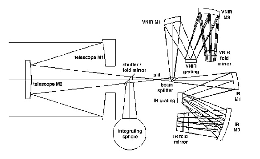
Before I could derive human perceptual color, I needed to perform a few preprocessing steps. The first issue I encountered was in CRISM's its sensitivity range. To cover as much of the spectrum as CRISM does, it actually needs three camera sensors. One of these sensors ('VIS') covers most of the visible spectrum. This sensor loses its sensitivity extending into the red and blue, in part because the silicon photodiode detectors are less sensitive to these wavelengths, and in part because these pixel rows are located near the edges of the sensor and are more prone to electronic noise. These noisy bands ('bad bands') were removed in the newer CRISM processing routine.These bad bands needed to be replaced, because they cover a portion of the visible range that the human eye is sensitive to. For the blue bad bands, I extrapolated a handful of additional channels from the existing blue bands. For the red bad bands, I used some bands from the near-infrared sensor ('NIR') to create new bands through interpolation.
The next thing was to feed the data into the human visual response functions. To accomplish this, I used a 'spectrum to sRGB colorspace' function described on the Scientific Python Blog, with a slight modification to match the axis values of the provided cone cell response functions to match the wavelength values of the CRISM band wavelengths. This process only preserves the chromaticity of the CRISM data - the variations in color in the images, not the luminance (relative brightnesses) of each pixel. To fix this, I created a luminance image by averaging every band measured by the VIS detector.
After finishing the human perceptual color portion of this code, I realized I had built a tool that could also be used for some other fun things. For example, if I wanted to see what the Martian surface looked like if human eyes were sensitive to a different set of wavelengths, I only needed to transplant the cone cell response functions to the spectral range I wanted. Another realization was that the response functions I had implemented were similar to the functions that describe color filter transmissions. If I wanted to simulate the color of the surface viewed through another color imager, like HiRISE or HRSC, I only needed a table describing the response function across a wavelength range. This made possible some interesting comparisons between the "visible color" produced by various spacecraft that have orbited Mars.
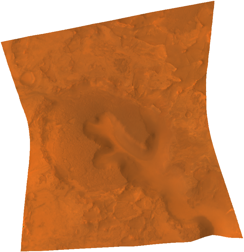
To review the results, I'm going to use a CRISM image from the Nili Fossae region. It shows a crater which has apparently been filled with lava flows, and then eroded by water. The raw output of the code looks about like what you would expect for a photo of Mars: slightly hazy, with a deep orange tint.
This looks a lot different from the CRISM visible color parameter released by the mission team, but it turns out they apply some color balancing to the image! This is understandable - at several points in the light's journey to the spacecraft, it has been filtered by Mars' dusty atmosphere, and that masks a lot of the color variations a human would be able to see if the surface was illuminated by white light. Let's color balance and compare.
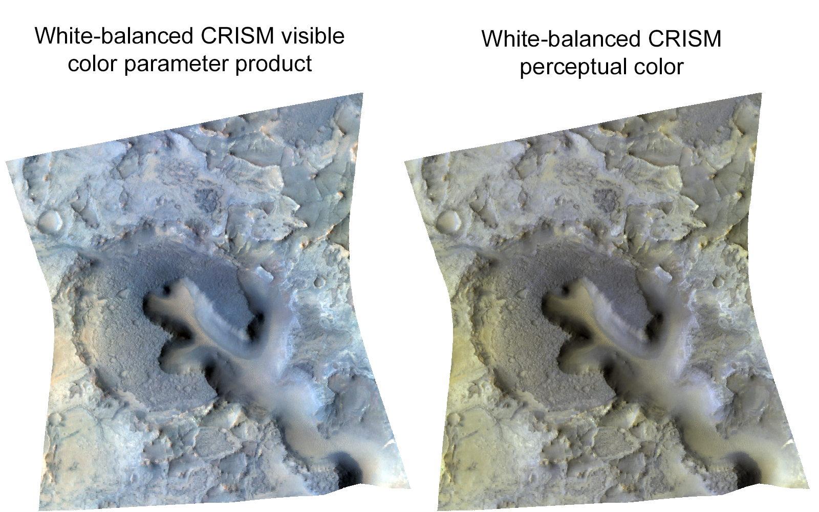
Looks reasonable! You can see that the perceptual color image overall is a little browner. I'm not entirely sure why this is, but I'll wager a guess: the wider sampling ranges in the perceptual color estimation are reducing the variation in intensity between channels. Basalts, like the kind present in this imaging scene, have a slight decrease in the amount of light they reflect from blue to red wavelengths. With the more limited sampling ranges in the CRISM visible color parameter product, the higher amount of blue light reflected is more strongly apparent, while in the perceptual color image these color differences are slightly reduced. Either way, it's a subtle difference.
When we make RGB color images from spacecraft data, the tendency is to not think much about the filters beyond their names. We'll use a filter labeled "blue" as the blue channel and "red" as the red channel. But in reality, the filters are different from spacecraft to spacecraft. The range of light let through a filter is different depending on the material it is constructed from, the thickness of the filter, and so on. This will slightly change the colors that we see when we make a photo from those filters. How do some of these diffferent imaging systems compare to one another? Here's a look at a few camera systems that have operated on Mars:
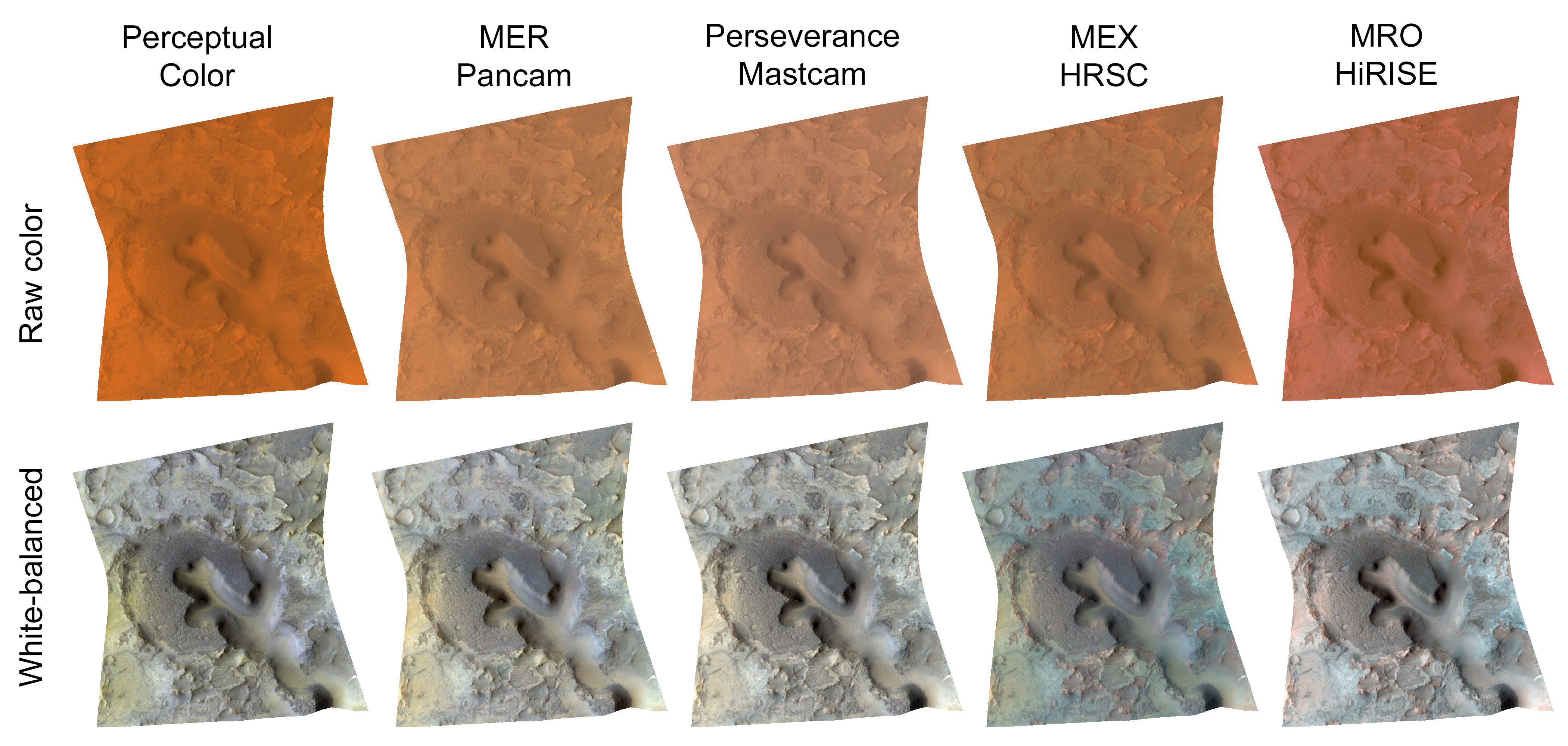
The largest differences are with Mars Express HRSC and Mars Reconnaissance Orbiter HiRISE images. It turns out that this difference is easy to explain: the red filters of these camera systems are at much redder wavelengths than the human eye. The human eye is relatively insensitive to wavelengths beyond 700 nm, but in both spacecraft, the red filter lets in the most light at around 800 nm. Depending on the mineral it is associated with, oxidized iron atoms strongly absorb light at various points in the 700-1400 nm range. HRSC and HiRISE are picking up shades of this iron absorption, leading to a greater variety of colors visible in the photo.
This begs the question: what would the human eye see if it were sensitive to this region of the spectra? I added a couple of lines of code to allow me to keep the same shape to the human color response functions, but shift the wavelengths around. Here is what the Nili Fossae region would look like if humans had infrared color vision, and could see wavelengths between 1100-1800 nm, which is where most minerals show their greatest variability in color:
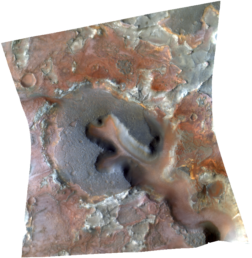
You can see a great deal of variability in the surface color. In general, reds in this image correspond to olivine, which more strongly absorbs light in the 1200 nm region, and blues correspond to pyroxene, which more strongly absorbs light in the 1600 nm region. However, these colors can be changed by the presence of other minerals, and identifying what those minerals are requires actually looking closely at the CRISM spectra.
I hope you enjoyed reading about this project! If you want to experiment with your own CRISM images, I have made the code available at my Github page. I'd like to give a quick thanks to Andrew Annex for his addition of a couple performance modifications to the code. Unfortunately, this code is not multi-platform, as the Rasterio package used for data input/output cannot read NASA's .img archival format. Converting to a format that can be read by Rasterio requires conversion to the .cub filetype used by the Linux-only USGS ISIS3 software. I am trying to figure out a way around this dependency and hopefully future releases of this code will be cross-platform!
Page last updated: June 11, 2022